LeNet in a nutshell
Hello There, First things first welcome to my Blog, I am Ritik Dutta and here in this blog i will show you how LeNet works, Architecture, how to train model using LeNet acchitecture on keras and a also how to design a better model than LeNet using same architecture but with different activation, loss functions etc, and compare the accuracy of new LeNet and original LeNet model.
LeNet was developed in 1998 by Yann Lecun. It was a major breakthrough in Deep Learning more specifically in Convolution Neural Networks Field, as it was the first CNN architecture.
LeNet was trained on MNIST dataset (A handwritten dataset for digit recognition).

LeNet Acchitecture

First Layer
in first layer we have input of 32*32 where we apply 6 filters of size 5*5, so the Output is 28*28.
28 because when we apply filters to each features of 32*32 image we get output as 28*28

We can also calculate this with a formula by (input size-kernal size)+1, where 1 is a bias. hence the output will be (32–5+1)=28.
We have Neurons as 28*28*6 = 4704.
And no. of trainable parameters as (5*5+1)*6 where 1 bieng a bias.
Trainable parameters are kernals like in an image there could be 100’s of features, we don’t need all of the features we need only dominating fratures so in CNN we extract those perticular parameters known as trainable parameters.
Also we have no. of connection as (5*5+1)*6*28*28 = 122304, hence each pixel is connected to 5*5 pixels and 1 bias so there are this no. of connections but we need to learn only 156 parameters, mainly through weight sharing.
Second Layer
similarly, We have
input of 28*28 where we apply Average Pooling of size 2*2 with stride = 2, so the Output is 14*14.
14 because when we apply pooling to each features of 28*28 image we get output as 28/2 (because the stride is 2).
We has Neurons as 14*14*6=1176.
And no. of trainable parameters as 2*6.
Also we have no. of connection as (2*2+1)*6*14*14 = 5880.
Third Layer
Similarly From above, We have
input = 14*14
convolution kernal size = 5*5
output = 10 (14–5+1)
trainable parameters =(5*5*6*10)+16 =1516
Fourth Layer
input = 10*10
convolution kernal size = 2*2
output = 5 (10/2)
trainable parameters = 32 (2*16)
Fifth Layer
this layer is responsible for flatterning the inputs from fourth layer.
input = all 16 unit feature map of fourth layer
convolution kernal size = 5*5
output = 120
trainable parameters = 48120 (120*(16*5*5+1))
Sixth Layer
This layer is fully connected layer and has 84 nodes.
Output Layer
This layer contains 10 nodes, for each numbers (0–9)
Training the Model
import keras
from keras.datasets import mnist
from keras.layers import Conv2D, MaxPooling2D
from keras.layers import Dense, Flatten
from keras.models import Sequential
Importing the libraries
(x_train, y_train), (x_test, y_test) = mnist.load_data(
Loading and Splitting dataset
x_train = x_train.reshape(x_train.shape[0], 28, 28, 1)
x_test = x_test.reshape(x_test.shape[0], 28, 28, 1)
Reshaping
x_train = x_train / 255
x_test = x_test / 255
Grey scaling images (Normalization)
y_train = keras.utils.to_categorical(y_train, 10)
y_test = keras.utils.to_categorical(y_test, 10)
One Hot Encoding
model = Sequential()
model.add(Conv2D(6, kernel_size=(5, 5), activation=’tanh’, input_shape=(28, 28, 1)))
Select 6 feature convolution kernels with a size of 5*5 (without offset). The size of each feature map is 32−5 + 1=28
That is, the number of neurons has been reduced from 1024 to 28 ∗ 28 = 784 .
Parameters between input layer and C1 layer: 6 ∗ (5 ∗ 5 + 1)
model.add(AveragePooling2D(pool_size=(2, 2)))
The input matrix size of this layer is 14 * 14 * 6, the filter size used is 5 * 5, and the depth is 16. This layer does not use all 0 padding, and the step size is 1.
The output matrix size of this layer is 10 * 10 * 16. This layer has 5 * 5 * 6 * 16 + 16 = 2416 parameters
model.add(Conv2D(16, kernel_size=(5, 5), activation=’tanh’))
The input matrix size of this layer is 10 * 10 * 16. The size of the filter used in this layer is 2 * 2, and the length and width steps are both 2, so the output matrix size of this layer is 5 * 5 * 16.
model.add(AveragePooling2D(pool_size=(2, 2)))
The input matrix size of this layer is 5 * 5 * 16. This layer is called a convolution layer in the LeNet-5 paper, but because the size of the filter is 5 * 5,
So it is not different from the fully connected layer. If the nodes in the 5 * 5 * 16 matrix are pulled into a vector, then this layer is the same as the fully connected layer.
The number of output nodes in this layer is 120, with a total of 5 * 5 * 16 * 120 + 120 = 48120 parameters.
model.add(Flatten())
model.add(Dense(120, activation=’tanh’))
The number of input nodes in this layer is 120 and the number of output nodes is 84. The total parameter is 120 * 84 + 84 = 10164 (w + b)
model.add(Dense(84, activation=’tanh’))
The number of input nodes in this layer is 84 and the number of output nodes is 10. The total parameter is 84 * 10 + 10 = 850
model.add(Dense(10, activation=’softmax’))
model.compile(loss=keras.metrics.categorical_crossentropy, optimizer=keras.optimizers.SGD(), metrics=[‘accuracy’])
model.fit(x_train, y_train, batch_size=128, epochs=20, verbose=1, validation_data=(x_test, y_test))
score = model.evaluate(x_test, y_test)
print(‘Test Loss:’, score[0])
print(‘Test accuracy:’, score[1])
Training with original Activation and loss function were available at that time
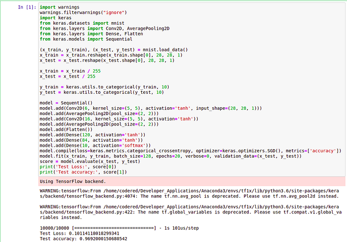
We are getting accuracy as 96% quite good but what if we use better activation and loss function for a perticular case which were present to out time? will the accuracy increase or decrease? lets see.
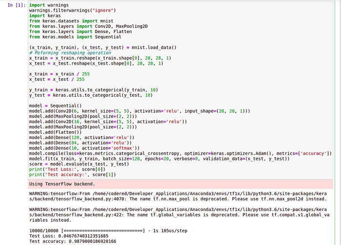
Vollah the accuracy has increased.
That is it for this blog hope u will understand the architecture and working of LeNet.